NLP - Topic Modeling (Python)

Purpose

For this project I have scraped (see my scraping tutorial here) news articles from Reuters and clustered them using Latent Dirichlet Allocation (LDA).

Since there is no proper classification of articles on Reuters, my model supports the reader in finding articles relating to a specific topic. Furthermore, the model could be used to classify future articles as well.

1 - Data Gathering

I used the scraper i described here to get all available Euro-Zone news from Reuters.

The data can be downloaded from here.

2 - Required Packages

import logging
logging.captureWarnings(True)

# Data Processing
from collections import Counter
import datetime as dt
from dateutil.relativedelta import relativedelta
import numpy as np
import pandas as pd

# Plotting
import matplotlib.pyplot as plt
%matplotlib inline
import pyLDAvis
import pyLDAvis.sklearn
from wordcloud import WordCloud

# NLP
import gensim
from nltk.stem import SnowballStemmer
from nltk.util import ngrams
import spacy

# Modeling
from sklearn.decomposition import LatentDirichletAllocation
from sklearn.feature_extraction.text import CountVectorizer
from sklearn.model_selection import GridSearchCV

3 - Data Cleaning

In this step i read the data into a pandas dataframe, clean missing values and convert dates stored in strings to actual dates.

3.1 - Custom Functions

def read_data_from_csv(path_to_data, sep=";"):
    df = pd.read_csv(path_to_data, sep=sep)
    print(f"shape of df: {df.shape}")
    print(f"columns in df: {list(df.columns)}")
    return df

def drop_rows_with_missing_values(df):
    rows_orig = df.shape[0]
    df = df.dropna().reset_index(drop=True)
    print(f"{rows_orig-df.shape[0]} rows dropped")
    print(f"new shape of df: {df.shape}")
    return df

def convert_date_ReutersNews(df, date_col):
    df = df[df.scraper == "reuters_news"].copy()
    month_map = {
        "January":1, "February":2, "March":3,
        "April":4, "May":5, "June":6,
        "July":7, "August":8, "September":9,
        "October":10, "November":11, "December":12
    }
    regex_date = r"([A-Z]\w+) (\d+), (\d+)"
    mdy = df[date_col].str.extract(regex_date)
    df["month"] = mdy[0].map(month_map)
    df["day"] = mdy[1]
    df["year"] = mdy[2]
    df[date_col] = pd.to_datetime(df[['year', 'month', 'day']])
    df = df.drop(['year', 'month', 'day'], axis=1).reset_index(drop=True)
    return df

def convert_dates(df, date_col):
    df_Reuters = convert_date_ReutersNews(df, date_col)
    df_full = pd.concat([df_Reuters])
    print(f"shape of df: {df_full.shape}")
    print(f"columns in df: {list(df_full.columns)}")
    return df_full

3.2 - Read Data

path_data = "../data/20200329_reuters_news_euro_zone.csv"
df = read_data_from_csv(path_data)

shape of df: (9773, 5)
columns in df: ['scraper', 'url', 'date', 'title', 'text']

df[["date", "title", "text"]].head(3)

	date	title	text
0	July 24, 2018 / 8:08 PM / in 3 months	Reuters Leadership	Jane Barrett Rob Cox...
1	March 28, 2020 / 4:15 PM / Updated 14 hours ago	Coronavirus death toll in Italy's Lombardy ris...	MILAN (Reuters) - The death toll from an outbr...
2	March 28, 2020 / 10:01 PM / Updated 10 hours ago	Northern Ireland brings in tough measures to f...	BELFAST (Reuters) - Northern Ireland will intr...

3.3 - Missing Value Treatment

I decided to drop all rows with missing values

df.isnull().sum()

scraper     0
url         0
date       54
title      54
text        1
dtype: int64

df = drop_rows_with_missing_values(df)

55 rows dropped
new shape of df: (9718, 5)

3.4 - Converting to Actual Dates

The scraped date has the following form: ‘Month DD, YYYY …’. Since this can’t be properly used as a date, I used RegEx to parse the date from these strings.

df.date.iloc[0]

'July 24, 2018 /  8:08 PM / in 3 months'

df = convert_dates(df, "date")

shape of df: (9718, 5)
columns in df: ['scraper', 'url', 'date', 'title', 'text']

df.date.iloc[0]

Timestamp('2018-07-24 00:00:00')

4 - Exploratory Data Analysis

In this step i looked at published articles over time and futher cleaned the data based on the graphical results. This step is mainly necessary, because over time some of the older news articles are no longer available.

4.1 - Custom Functions

def keep_only_articles_published_after(df, date_col, date_min):
    rows_orig = df.shape[0]
    df = df[df[date_col] >= date_min].copy().reset_index(drop=True)
    print(f"{rows_orig-df.shape[0]} rows dropped")
    print(f"new shape of df: {df.shape}")
    return df

4.2 - Further Data Cleaning based on Publication Date

df_plot = df.date.value_counts().sort_index().reset_index()
df_plot.columns = ["date", "articles"]

fig = plt.figure(figsize=(20,3))
plt.hist(df_plot.date, bins=(df_plot.date.max()-df_plot.date.min()).days+1)
plt.title('Dates w/o Publications', fontsize=24)
plt.xlabel('publication date')
plt.gca().axes.get_yaxis().set_visible(False)
plt.show()

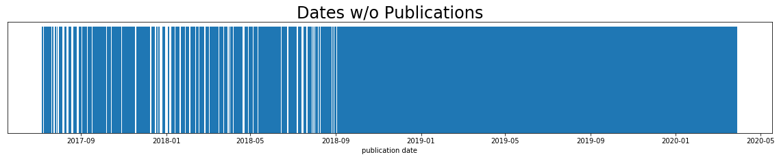
This plot clearly shows that some articles published before 09/2018 are no longer available online. The next graphic confirms this.

fig = plt.figure(figsize=(20,3))
plt.plot(df_plot.date, df_plot.articles)
plt.title('Published Articles over Time', fontsize=24)
plt.xlabel('publication date')
plt.ylabel('articles')
plt.show()

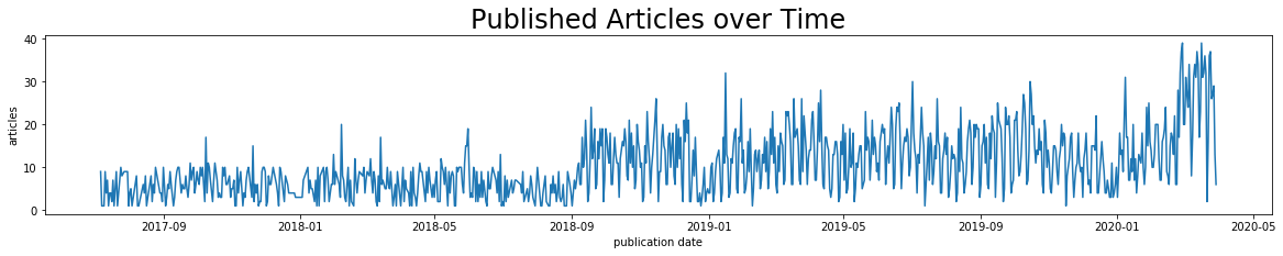
I have decided to not consider articles before September 2018 for this project.

date_min = dt.datetime(2018,9,1)
df = keep_only_articles_published_after(df, "date", date_min)

2000 rows dropped
new shape of df: (7718, 5)

After all these steps we reduced numbers of articles by 2,055 and are left with 7,718 articles over a time period of 1.5 years.

5 - Feature Engineering

I performed the following steps for feature engineering and text-data cleaning:

• Special character replacement
• Tokenization using gensim.utils.simple_preprocess
• Most of the articles have the following beginning: “Some-City (Reuters) - “. I decided to remove this pre-article information by searching for “reuters” and deleting all tokens before this keyword
• Lemmatization with POS-tagging using spacy’s “en_core_web_lg” (optional)
• Stemming using nltk’s “SnowballStemmer” (optional)
• Removing short words (min. word length can be specified) and stop-words
• Adding N-Grams (optional)

5.1 - Custom Functions

def remove_shortest_longest_articles(tokens, remove_lowest, remove_highest):
    orig_shape = tokens.shape
    article_length = tokens.apply(lambda x: len(x))
    article_length_vc = article_length.value_counts().sort_index().cumsum()/tokens.shape[0]
    remove_len = article_length_vc[(article_length_vc <= remove_lowest) | (1-article_length_vc <= remove_highest)].index
    tokens = tokens[~np.isin(article_length, remove_len)] # .reset_index(drop=True)
    print(f"{orig_shape[0]-tokens.shape[0]} articles dropped.")
    print(f"{tokens.shape[0]} articles remaining for modeling.")
    return tokens

5.2 - Create Final Tokens for Modeling

def preprocess_text(txt,
                    spacy_lang_obj,
                    min_word_length=3,
                    lemmatize=True,
                    stem=True,
                    ngrams_n_list=[2]):
    """
    Preprocessing of text/titles
    Input:
        - txt: string - text/title
        - spacy_lang_obj = spacy.load("en_core_web_XX")
        - min_word_length: integer - keep only words with length >= min_word_length
        - lemmatize: boolean - if True then lemmatize tokens
        - stem: boolean - if True then stem tokens
        - ngrams_n_list - list of integers, if ngrams not wanted, pass empty list []
    """

    # spacy language tokenizer, tagger, parser, ner and word vectors
    nlp = spacy_lang_obj

    # replace special characters
    special_chars = {"ö":"oe", "ä":"ae", "ü":"ue", "ß":"ss"}
    for char in special_chars:
        txt = txt.replace(char,special_chars[char])

    # split text into tokens
    tokens = gensim.utils.simple_preprocess(txt, deacc=True)

    # remove pre-article information (mostly cities)
    ind_reuters = tokens.index("reuters") if "reuters" in tokens else -1
    if ind_reuters > 5:
        ind_reuters = -1
    tokens = tokens[ind_reuters+1:]
    
    # lemmatize tokens using spacy
    if lemmatize == True:
        full_text = nlp(" ".join(tokens))
        tokens = [token.lemma_ for token in full_text if token.pos_ in ['NOUN', 'ADJ', 'VERB', 'ADV']]

    # stem tokens using SnowballStemmer from nltk
    if stem == True:
        stemmer = SnowballStemmer('english')
        tokens = [stemmer.stem(token) for token in tokens]

    # keep only tokens with length >= min_word_length
    tokens = [token for token in tokens if len(token) >= min_word_length]

    # remove stop-words from tokens
    tokens_wo_stopwords = []
    for token in tokens:
        if (nlp.vocab[token].is_stop == False) & (~np.isin(token, ["reuters", "reuter"])):
            tokens_wo_stopwords.append(token)

    # build n-grams
    ngram_list = []
    if ngrams_n_list != []:
        for n in ngrams_n_list:
            if n > 1:
                for ngram in ngrams(tokens_wo_stopwords, n):
                    ngram_list.append("_".join(str(i) for i in ngram))

    # final list of tokens
    tokens_final = tokens_wo_stopwords + ngram_list

    return tokens_final

Load Spacy’s pretrained statistical model for English.

nlp = spacy.load("en_core_web_lg")

For my model I decided to

• set min_word_length to 3,
• skip stemming and
• use bigrams.

tokens_final = df.text.apply(
    lambda x: preprocess_text(
        txt=x,
        spacy_lang_obj=nlp,
        min_word_length=3,
        lemmatize=True,
        stem=False,
        ngrams_n_list=[2]
    )
)

tokens_final.head(3)

0    [death, toll, outbreak, coronavirus, northern,...
1    [introduce, sweeping, new, power, combat, spre...
2    [team, minister, win, test, coronavirus, sympt...
Name: text, dtype: object

5.3 - Publication-Length: Outlier Treatment

Note that the lengths include bigrams as well

tokens_len = tokens_final.apply(lambda x: len(x))

print(f"min. publication length: {min(tokens_len)}")
print(f"max. publication length: {max(tokens_len)}")

min. publication length: 7
max. publication length: 5281

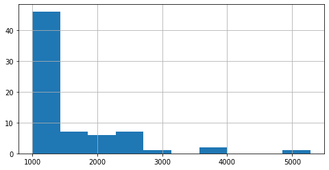
Looking at the distribution of articles-lengths yields the following (for the plot I excluded articles with >1,000 words):

fig = plt.figure(figsize=(8, 4))
tokens_len[tokens_len <= 1000].hist(bins=200)
plt.show()

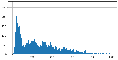
fig = plt.figure(figsize=(8, 4))
tokens_len[tokens_len <= 100].hist(bins=40)
plt.show()

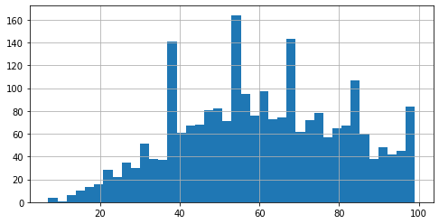
fig = plt.figure(figsize=(8, 4))
tokens_len[tokens_len > 1000].hist()
plt.show()

Based on the above and further analysis I have decided to exclude the top 1% of the short/longest articles. This leaves us with 7580 publications for modeling.

tokens_final = remove_shortest_longest_articles(tokens_final, 0.01, 0.01)

138 articles dropped.
7580 articles remaining for modeling.

5.4 - Vocabulary

We now have a look at the vocabulary we will later pass to the model.

# split vocabulary into uni- and bi-grams
unigrams = [word for words in tokens_final for word in words if not "_" in word]
bigrams = [word for words in tokens_final for word in words if "_" in word]

print(f"total number of words: {len(unigrams)}")
print(f"total number of bigrams: {len(bigrams)}")

total number of words: 1027221
total number of bigrams: 1019657

# unique words and bigrams in our train-dataset
unigrams_unique = sorted(list(set(unigrams)))
bigrams_unique = sorted(list(set(bigrams)))
print(f"unique words: {len(unigrams_unique)}")
print(f"unique bigrams: {len(bigrams_unique)}")

unique words: 17957
unique bigrams: 577945

most_used_unigrams = pd.DataFrame.from_dict(Counter(unigrams), orient="index").reset_index()
most_used_unigrams.columns = ["word", "occurence"]
most_used_unigrams.sort_values(by="occurence", inplace=True)
most_used_unigrams.tail(5)

	word	occurence
1029	percent	4685
135	tell	4708
620	deal	5514
61	government	7004
203	year	10035

most_used_bigrams = pd.DataFrame.from_dict(Counter(bigrams), orient="index").reset_index()
most_used_bigrams.columns = ["word", "occurence"]
most_used_bigrams.sort_values(by="occurence", inplace=True)
most_used_bigrams.tail(5)

	word	occurence
199	news_conference	476
2370	central_bank	588
3211	year_old	656
8371	interest_rate	776
598	tell_reporter	862

wordcloud_unigrams = WordCloud(
    width=3000,
    height=1000, 
    background_color="white", 
    min_font_size = 12
).generate(" ".join(unigrams))

fig = plt.figure(figsize=(15, 5))
plt.imshow(wordcloud_unigrams)
plt.axis("off")
plt.tight_layout(pad=0)

6 - Modeling

6.1 - Create Document-Term Matrix

corpus = tokens_final.apply(lambda x: " ".join(x))

# only count words that appear in more than 15 articles
# don't count words that appear in more than 75% of articles
cv = CountVectorizer(min_df=15, max_df=0.75)

document_term_matrix = cv.fit_transform(corpus)

6.2 - Baseline Model

lda_baseline = LatentDirichletAllocation(n_jobs=-1).fit(document_term_matrix)

print("------ Baseline Model ------")
# print(f"perplexity: {round(lda_baseline.perplexity(document_term_matrix),2)}") # see comment in 6.3.2
print(f"log_likelihood: {round(lda_baseline.score(document_term_matrix),2)}")

------ Baseline Model ------
log_likelihood: -8421569.0

6.3 - Grid-Search to find optimal parameters

6.3.1 - Log-Likelihood

topic_models_ll = GridSearchCV(
    estimator=LatentDirichletAllocation(n_jobs=-1),
    param_grid={"n_components": list(range(10, 41, 2)),
                "learning_decay": [0.5, 0.7, 0.9]},
    cv=[(slice(None), slice(None))], # no cv for unsupervised ml
    n_jobs=-1,
    verbose=20
)

topic_models_ll.fit(document_term_matrix)

print("---------------- Best Model (Log-Likelihood) ----------------")
print(f"model parameters: {topic_models_ll.best_params_}")
# print(f"perplexity: {round(topic_models_ll.best_estimator_.perplexity(document_term_matrix),2)}") # see comment in 6.3.2
print(f"log_likelihood: {round(topic_models_ll.best_estimator_.score(document_term_matrix),2)}")

---------------- Best Model (Log-Likelihood) ----------------
model parameters: {'learning_decay': 0.5, 'n_components': 28}
log_likelihood: -8385793.37

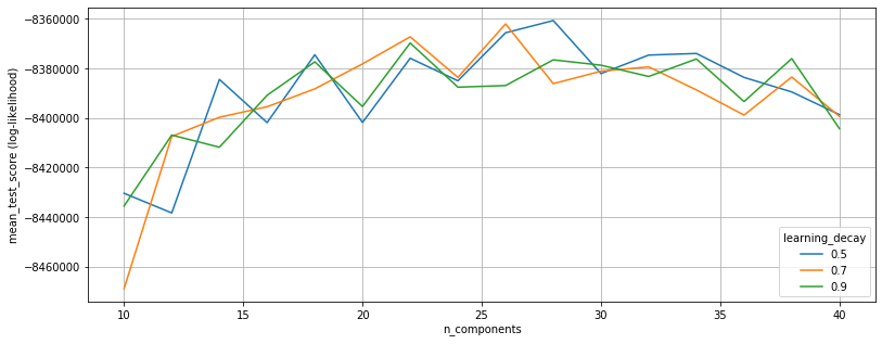
models_ll = pd.DataFrame(topic_models_ll.cv_results_)
models_ll = models_ll[["param_learning_decay", "param_n_components", "mean_test_score"]]
models_ll.rename(columns={'mean_test_score':'log_likelihood'}, inplace=True)
models_ll.sort_values(by="log_likelihood", ascending=False, inplace=True)

# top models (log likelihood)
models_ll.head(5)

	param_learning_decay	param_n_components	log_likelihood
9	0.5	28	-8.360676e+06
24	0.7	26	-8.362038e+06
8	0.5	26	-8.365602e+06
22	0.7	22	-8.367235e+06
38	0.9	22	-8.369719e+06

df_plot = pd.DataFrame(topic_models_ll.cv_results_)

n_topics = list(range(10,41,2))

ld5 = df_plot[(df_plot.param_learning_decay==0.5)].mean_test_score.tolist()
ld7 = df_plot[(df_plot.param_learning_decay==0.7)].mean_test_score.tolist()
ld9 = df_plot[(df_plot.param_learning_decay==0.9)].mean_test_score.tolist()

plt.figure(figsize=(13, 5))
plt.plot(n_topics, ld5, label="0.5")
plt.plot(n_topics, ld7, label="0.7")
plt.plot(n_topics, ld9, label="0.9")
plt.xlabel("n_components")
plt.ylabel("mean_test_score (log-likelihood)")
plt.legend(title='learning_decay', loc='lower right')
plt.grid()
plt.show()

6.3.2 - Perplexity

Extend the LDA class in order to use perplexity as score. Currently not possible, as there seems to be a bug in sklearn.

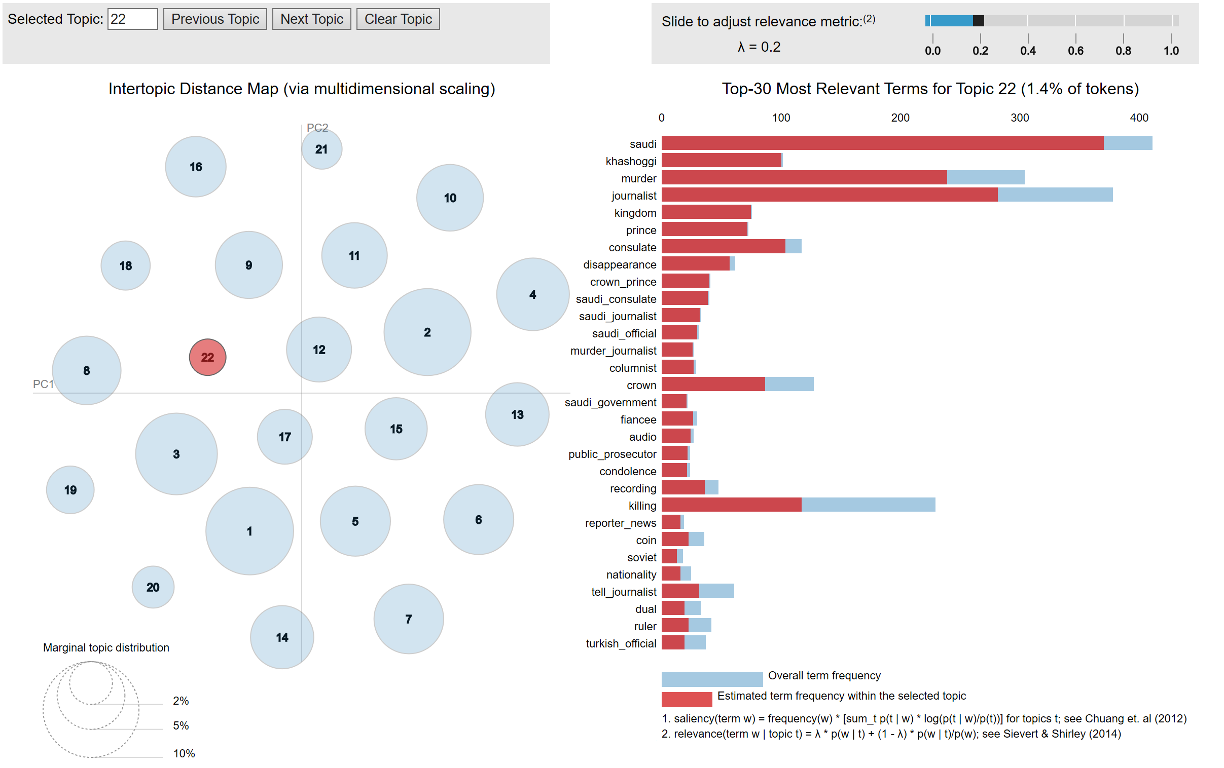
6.4 - Model Choice and Visualization

I decided to not go with the model suggested via Grid-Search and chose the model with n_components=22 and learning_decay=0.7 instead (4th-best model). The main reason for this is that the difference to a model with more topics (28 in the best case) is not too significant.

lda_final = LatentDirichletAllocation(
    n_components=22,
    learning_decay=0.7,
    n_jobs=-1
).fit(document_term_matrix)

I used pyLDAvis for visualization purposes. I have saved the results as HTML and they can be viewed here.

pyLDAvis.enable_notebook()
panel = pyLDAvis.sklearn.prepare(lda_final, document_term_matrix, cv, mds='tsne')
pyLDAvis.save_html(panel, 'lda_final.html')

7 - Final Dataframe including Topic

topic = np.argmax(lda_final.transform(document_term_matrix), axis=1)+1

tok_cor_top = pd.DataFrame(
    data={"corpus": corpus, "tokens": tokens_final, "topic": topic},
    index=corpus.index
)

df_topics = df.merge(tok_cor_top, left_index=True, right_index=True, how="inner").reset_index(drop=True)

df_topics[["date", "title", "text", "topic"]].head()

	date	title	text	topic
0	2020-03-28	Coronavirus death toll in Italy's Lombardy ris...	MILAN (Reuters) - The death toll from an outbr...	12
1	2020-03-28	Northern Ireland brings in tough measures to f...	BELFAST (Reuters) - Northern Ireland will intr...	12
2	2020-03-27	British ministers won't be tested for virus un...	LONDON (Reuters) - Boris Johnson’s top team of...	12
3	2020-03-27	Johnson's central role to UK virus response en...	LONDON (Reuters) - People with a central role ...	12
4	2020-03-27	Foreigners face suspicion in China as coronavi...	SHENZHEN, China/SHANGHAI (Reuters) - Francesca...	12